Striking a Balance: Exploring Fairness in Buffer Allocation and Packet Scheduling

Striking a Balance: Exploring Fairness in Buffer Allocation and Packet Scheduling

Recently, I’ve been contemplating the concept of fairness, and I see interesting parallels between being a parent and being a network professional. As human beings, we have an inherent, intuitive sense of fairness that manifests itself in various everyday situations. Let me illustrate this idea with a couple of hypothetical scenarios:

Scenario 1: Imagine I’m a parent with four young children, and I’ve ordered a pizza for them to share. If I want to divide the pizza fairly among the children, fairness would mean that each child receives an equal portion - in this case, one-quarter of the pizza.

Scenario 2: Now let’s say I’ve ordered another pizza for the same four children, but one of the kids only cares for pizza a little and will only eat one-tenth of his share. In this situation, it wouldn’t be fair for me to give that child who doesn’t like pizza more than one-tenth of the piece because the excess would go to waste. The fair way to divide the pizza would be to give the child who doesn’t like pizza a one-tenth portion and split the remaining nine-tenths evenly among the other three kids.

The approach mentioned in the second scenario Continue reading

Back to Basics: A Primer on Communication Fundamentals

Motivation

In our rapidly advancing world, communication speeds are increasing at a fast pace. Transceiver speeds have evolved from 100G to 400G, 800G, and soon even 1.6T. Similarly, Optical systems are evolving to keep up with the pace. If we dig deeper, we will discover that many concepts are shared across various domains, such as Wi-Fi, optical communications, transceivers, etc. Still, without the necessary background, It’s not easy to identify the patterns. If we have the essential knowledge, it becomes easier to understand the developments happening in the respective areas, and we can better understand the trade-offs made by the designers while designing a particular system. And that’s the motivation behind writing this post is to cover fundamental concepts which form the basis for our modern communication system and how they all relate to each other.

Waves

So let’s start with the most fundamental thing, i.e., wave. A wave is a disturbance that carries energy from one location to another without displacing matter. Waves transfer energy from their source and do not cause any permanent displacement of matter in the medium they pass through. The following animation demonstrates this concept.

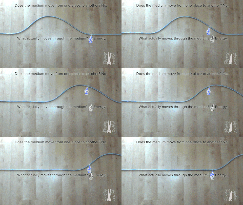
Ocean and sound waves are mechanical waves Continue reading

Back to Basics: A Primer on Communication Fundamentals

Gravity Model

Motivation

I recently read Google’s latest sigcomm paper: Jupiter Evolving on their Datacenter fabric evolution. It is an excellent paper with tons of good information, and the depth and width show what an engineering thought process should look like. The central theme talks about the challenges faced with deploying and scaling Clos fabrics and how they have evolved by replacing the spine layer with OCS that allows the blocks to be directly connected, calling it Direct connect topology.

If you look closely, the Direct Connect topology resembles Dragonfly+, where you have directly connected blocks.

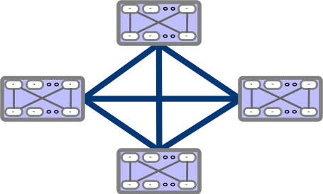
The paper has many interesting topics, including Traffic and Topology Engineering and Traffic aware routing. One of the most exciting parts to me, which will be understandably missing, is the formulation of Traffic engineering problems as Optimization problems. I would love to see some pseudo-real-world code examples made publicly available.

However, one thing that surprised me the most was from a Traffic characteristics perspective, a Gravity model best described Google’s Inter-Block traffic. When I studied Gravity Model, I thought this was such a simplistic model that I would never see that in real life, but it turns out I was wrong, and it still has practical Continue reading

Gravity Model

Routing Protocol Implementation Evaluation in Fat-Trees

Network design discussions often involve anecdotal evidence, and the arguments for preferring something follow up with “We should do X because at Y place, we did this.”. This is alright in itself as we want to bring the experience to avoid repeating past mistakes in the future. Still, more often than not, it feels like we have memorized the answers and without reading the question properly, we want to write down the answer vs. learning the problem and solution space, putting that into the current context we are trying to solve with discussions about various tradeoffs and picking the best solution in the given context. Our best solution for the same problem may change as the context changes. Also, this problem is everywhere. For example: Take a look at this twitter thread

Maybe one way to approach on how to think is to adopt stochastic thinking and add qualifications while making a case if we don’t have all the facts. The best engineers I have seen do apply similar thought processes. As world-class poker player Annie Duke points out in Thinking in Bets, even if you start at 90%, your ego will have a much easier time with Continue reading

Routing Protocol Implementation Evaluation in Fat-Trees

Steady State Markov Process

A Markov chain or Markov process is a stochastic model describing a sequence of possible events in which the probability of each event depends only on the state attained in the previous event. It is named after the Russian mathematician Andrey Markov.

Markov chains help model many real-word processes, such as queues of customers arriving at the airport, queues of packets arriving at a Router, population dynamics. Please refer to this link for a quick intro to Markov chains.

Problem

Let’s use a simple example to illustrate the use of Markov Chains. Assume that you own a barber shop, and You notice that Customers don’t wait if there is no room in the waiting room and will take their business elsewhere. You want to invest to avoid this, and you have the following info in hand:

• You have two barber chairs and two barbers.
• You have a waiting room for four people.
• You usually observe 10 Customers arriving per hour.
• Each barber takes about 15mins to serve a single customer. So each barber can serve four customers per hour.

You have finite space in the shop, so add two more chairs in the waiting room or add another barber. Now Continue reading

Steady State Markov Process

Linear Discriminant Analysis Rough Notes

Linear Discriminant Analysis Rough Notes

Linear Discriminant Analysis (LDA)

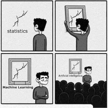
LDA is an alternative way to predict $Y$, based on partitioning the explanatory variable into two sets: one set prediction is $\hat{Y}=1$ or $\hat{Y}=0$ in the other set. Approach here is to model the distribution of $X$ in each of the classes separately, and then use Bayes Theorem to obtain $P(Y |X)$.

Unlike Logistic regression, LDA treats explanatory variables as independent Random Variables, $X = (X_{1},…,X_{p})$. Assuming common covariance matrix for $X$ within each $Y$ category, Ronald Fisher derived the linear predictor of explanatory variables such that its observed values when $y=1$ were seperated as much as possible from its values when $y=0$, relative to the variability of the linear predictor values within each $y$ category. This linear predictor is called Linear Discriminant function. Using Gauassian distribution for each class, leads to linear or quadratic discriminant analysis. We can express the linear probabilty model as:

$ E(Y|x) = P(Y=1|x) = \beta_{0}+\beta_{1}x_{1}+…+\beta_{p}x_{p} $

We can rewrite the below Bayes Theorem:

$ P(Y=1|x) = \frac{P(x|y=1).P(Y=1)}{P(x)} $

as

$ P(Y=1|x) = \frac{\hat{f}(x|y=1)P(Y=1)}{\hat{f}(x|y=1)P(Y=1)+\hat{f}(x|y=0)P(Y=0)} $

Discriminant Analysis is useful for:

• When the classes are well-separated, the parameter estimates for the logistic regression model are surprisingly unstable. Linear discriminant analysis does Continue reading

Generalized Linear Models(GLMs) Rough Notes

Generalized Linear Models(GLMs) Rough Notes

Generalized Linear Model

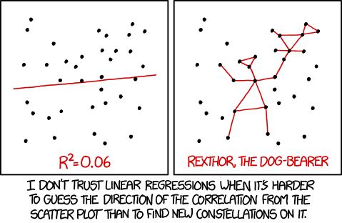
In case of Linear Models, we assume a linear relationship between the mean of the response variable and a set of explanatory variables with inference assuming that response variable has a Normal conditional distribution with constant variance. The Generalized Linear Model permits the distribution for the Response Variable other than the normal and permits modeling of non-linear functions of the mean. Linear models are special case of GLM.

GLM extends normal linear models to encompass non-normal distributions and equating linear predictors to nonlinear functions of the mean. The fundamental preimise is that

1) We have a linear predictor. $\eta_{i} = a + Bx$.

2) Predictor is linked to the fitted response variable value of $Y_{i}, \mu_{i}$

3) The linking is done by the link function, such that $g(\mu_{i}) = \eta_{i} $. For example, for a linear function $\mu_{i} = \eta_{i}$, for an exponential function, $log(\mu_{i}) = \eta_{i}$

$ g(\mu_{i}) = \beta_{0} + \beta_{1}x_{i1} + … + \beta_{p}x_{ip} $

The link function $g(\mu_{i})$ is called the link function.

Some common examples:

• Identity: $\mu = \eta$, example: $\mu = a + bx$
• Log: $log(\mu) = \eta$, example: $\mu = e^{a + bx}$
• Logit: $logit(\mu) = \eta$, example: $\mu = Continue reading

Linear Regression Rough Notes

Linear Regression Notes

Introduction

When it comes to stats, one of the first topics we learn is linear regression. But most people don’t realize how deep the linear regression topic is, and observing blind applications in day-to-day life makes me cringe. This post is not about virtue-signaling(as I know some areas I haven’t explored myself), but to share my notes which may be helpful to others.

Linear Model

A basic stastical model with single explanatory variable has equation describing the relation between x and the mean $\mu$ of the conditional distribution of Y at each value of x.

$ E(Y_{i}) = \beta_{0} + \beta_{1}x_{i} $

Alternative formulation for the model expresses $Y_{i}$

$ Y_{i} = \beta_{0} + \beta_{1}x_{i} + \epsilon_{i} $

where $\epsilon_{i}$ is the deviation of $Y_{i}$ from $E(Y_{i}) = \beta_{0} + \beta_{1}x_{i} + \epsilon_{i}$ is called the error term, since it represents the error that results from using the conditional expectation of Y at $x_{i}$ to predict the individual observation.

Least Squares Method

For the linear model $E(Y_{i}) = \beta_{0} + \beta_{1}x_{i}$, with a sample of n observations the least squares method determines the value of $\hat{\beta_{0}}$ and $\hat{\beta_{1}}$ that minimize the sum of squared residuals.

$ \sum_{i=1}^{n}(y_{i}-\hat{\mu_{i}})^2 = \sum_{i=1}^{n}[y_{i}-(\hat{\beta_{0}} + Continue reading

Linear Regression Rough Notes

Introduction

When it comes to stats, one of the first topics we learn is linear regression. But many people don’t realize how deep the linear regression topic is. Below are my partial notes on Linear Regression for anyone who may find this helpful.

Linear Model

A basic statistical model with single explanatory variable has equation describing the relation between x and the mean $\mu$ of the conditional distribution of Y at each value of x.

$ E(Y_{i}) = \beta_{0} + \beta_{1}x_{i} $

Alternative formulation for the model expresses $Y_{i}$

$ Y_{i} = \beta_{0} + \beta_{1}x_{i} + \epsilon_{i} $

where $\epsilon_{i}$ is the deviation of $Y_{i}$ from $E(Y_{i}) = \beta_{0} + \beta_{1}x_{i} + \epsilon_{i}$ is called the error term, since it represents the error that results from using the conditional expectation of Y at $x_{i}$ to predict the individual observation.

Least Squares Method

For the linear model $E(Y_{i}) = \beta_{0} + \beta_{1}x_{i}$, with a sample of n observations the least squares method determines the value of $\hat{\beta_{0}}$ and $\hat{\beta_{1}}$ that minimize the sum of squared residuals.

$ \sum_{i=1}^{n}(y_{i}-\hat{\mu_{i}})^2 = \sum_{i=1}^{n}[y_{i}-(\hat{\beta_{0}} + \hat{\beta_{1}}x_{i})]^2 = \sum_{i=1}^{n}e^{2}_{i} $

As a function of model parameters $(\beta_{0} , \beta_{1})$, the expression is quadratic in $\beta_{0},\beta_{1}$

$ Continue reading

Experimenting TCP Congestion Control(WIP)

Introduction

I have always found TCP congestion control algorithms fascinating, and at the same time, I know very little about them. So once in a while, I will spend some time with the hope of gaining some new insights. This blog post will share some of my experiments with various TCP congestion control algorithms. We will start with TCP Reno, then look at Cubic and ends with BBR.I am using Linux network namespaces to emulate topology for experimentation, making it easier to run than setting up a physical test bed.

TCP Reno

For many years, the main algorithm of congestion control was TCP Reno. The goal of congestion control is to determine how much capacity is available in the network, so that source knows how many packets it can safely have in transit (Inflight). Once a source has these packets in transit, it uses the ACK’s arrival as a signal that packets are leaving the network, and therefore it’s safe to send more packets into the network. By using ACKs for pacing the transmission of packets, TCP is self-clocking. 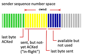The number of packets which TCP can inject into the network is controlled by Congestion Window(cwnd).

Congestion Window:

Continue reading

IS-IS Area proxy (WIP)

Introduction

Following up on the last post, we will explore IS-IS Area Proxy in this post. The main goal of the IS-IS Area proxy is to provide abstraction by hiding the topology. Looking at our toy topology, we see that we have fabrics connected, and the whole network is a single flat level-2 flooding domain. The edge nodes are connected at the ends, transiting multiple fabrics, and view all the nodes in the topology.

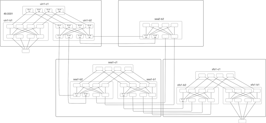
Now assume that we are using a router with a radix of 32x100G and want to deploy three-level Fat-Tree(32,3). For a single fabric, we will have 1280 nodes, 512 leaf Nodes, providing a bandwidth of 819T. If we deploy ten instances of this fabric, we are looking at a topology size greater than >12k Nodes. This is a lot for any IGP to handle. This inflation of Nodes (and links) is coming from deploying this sort of dense topology to provide more bandwidth and directly impacts IGP scaling in terms of Flooding, LSDB size, SPF runtimes, and frequency of SPF run.

Referring back to our toy topology, if we look from the edge node’s perspective, they use these fabrics as transit, and if we can Continue reading

IS-IS Average Flooding Rate

Introduction

In recent years, a lot of work has been done to scale IGPs for dense topologies, making IGPs again an interesting area. In this blog post, we will look at IS-IS Flooding and how we can measure the flooding rate, and in the future post explore Dynamic Flooding and Area Proxy.

Topology Setup

For our experiment, we will use a stripped-down topology connecting Four locations. The devices are emulated using Arista cEOS, and all devices are part of a single level2 flooding domain. Topology creation was done with the help of netsim-tools and containerlabs. So my regards go to everyone involved with the tool, as it took care of the monotonous work like IP-Addressing, wiring, and base configs.

In the above diagram, Nodes under uin1-b2 will be the primary focus of our deep dive. Node Label consists of the node name suffix and the last octet of the loopback IP. For example:

uin1-b2-t1-r1 with LSP ID of 0000.0000.0013 is highlighted as t1-r1(13) under uin1-b2 block.
uin1-b2-t2-r1 with LSP ID of 0000.0000.0009 is highlighted as t2-r1(09) under uin1-b2 block.

IS-IS Refresher

Let’s do a quick IS-IS refresher. We know that IS-IS Packets are of following types:

1. Continue reading