Leveling up Workers AI: general availability and more new capabilities
This post is also available in 简体中文, 繁體中文, 日本語, 한국어, Deutsch, Français and Español.

Welcome to Tuesday – our AI day of Developer Week 2024! In this blog post, we’re excited to share an overview of our new AI announcements and vision, including news about Workers AI officially going GA with improved pricing, a GPU hardware momentum update, an expansion of our Hugging Face partnership, Bring Your Own LoRA fine-tuned inference, Python support in Workers, more providers in AI Gateway, and Vectorize metadata filtering.
Workers AI GA
Today, we’re excited to announce that our Workers AI inference platform is now Generally Available. After months of being in open beta, we’ve improved our service with greater reliability and performance, unveiled pricing, and added many more models to our catalog.
Improved performance & reliability
With Workers AI, our goal is to make AI inference as reliable and easy to use as the rest of Cloudflare’s network. Under the hood, we’ve upgraded the load balancing that is built into Workers AI. Requests can now be routed to more GPUs in more cities, and each city is aware of the total available capacity for AI inference. If the request Continue reading
Running fine-tuned models on Workers AI with LoRAs
This post is also available in 简体中文, 繁體中文, 日本語, 한국어, Deutsch, Français and Español.

Inference from fine-tuned LLMs with LoRAs is now in open beta
Today, we’re excited to announce that you can now run fine-tuned inference with LoRAs on Workers AI. This feature is in open beta and available for pre-trained LoRA adapters to be used with Mistral, Gemma, or Llama 2, with some limitations. Take a look at our product announcements blog post to get a high-level overview of our Bring Your Own (BYO) LoRAs feature.
In this post, we’ll do a deep dive into what fine-tuning and LoRAs are, show you how to use it on our Workers AI platform, and then delve into the technical details of how we implemented it on our platform.
What is fine-tuning?
Fine-tuning is a general term for modifying an AI model by continuing to train it with additional data. The goal of fine-tuning is to increase the probability that a generation is similar to your dataset. Training a model from scratch is not practical for many use cases given how expensive and time consuming they can be to train. By fine-tuning an existing pre-trained model, Continue reading
Using wemulate with netlab
An RSS hiccup brought an old blog post from Urs Baumann into my RSS reader. I’m always telling networking engineers that it’s essential to set up realistic WAN environments when testing distributed software, and wemulate (a nice tc front-end) seemed like a perfect match. Even better, it runs in a container – an ideal component for a netlab-generated virtual WAN network.
wemulate acts as a bump in the wire; it uses Linux bridges to connect two container interfaces. We’ll use it to introduce jitter into an IP subnet:
┌──┐   ┌────────┐   ┌──┐
│h1├───┤wemulate├───┤h2│
└──┘   └────────┘   └──┘
◄──────────────────────►
     192.168.33.0/24
1000BASE-T Part 2 – Deepdive
In 1000BASE-T Part 1, we reviewed the layers and what their purpose is. Now we’re going to go much deeper into the layers that relate to the PHY, which is PCS, PMA, and Autonegotiation. First though, let’s review the objectives of 1000BASE-T:
- Support the CSMA/CD MAC.
- Comply with specifications for GMII (Clause 35).
- Support 1000 Mbit/s repeater (Clause 41).
- Provide line transmission support full and half duplex operation.
- Meet or exceed FCC Class A/CISPR or better operation.
- Support operation over 100 meters of copper balanced cabling (defined in 40.7).
- Bit Error Ratio less than or equal to 10^-10.
- Support Auto negotiation (Clause 28).
How does 1000BASE-T achieve a bandwidth of 1000 Mbit/s? As you probably know, the twisted pair cable consists of four pairs, eight wires in total, where transmit and receive are separated to achieve full duplex operation:
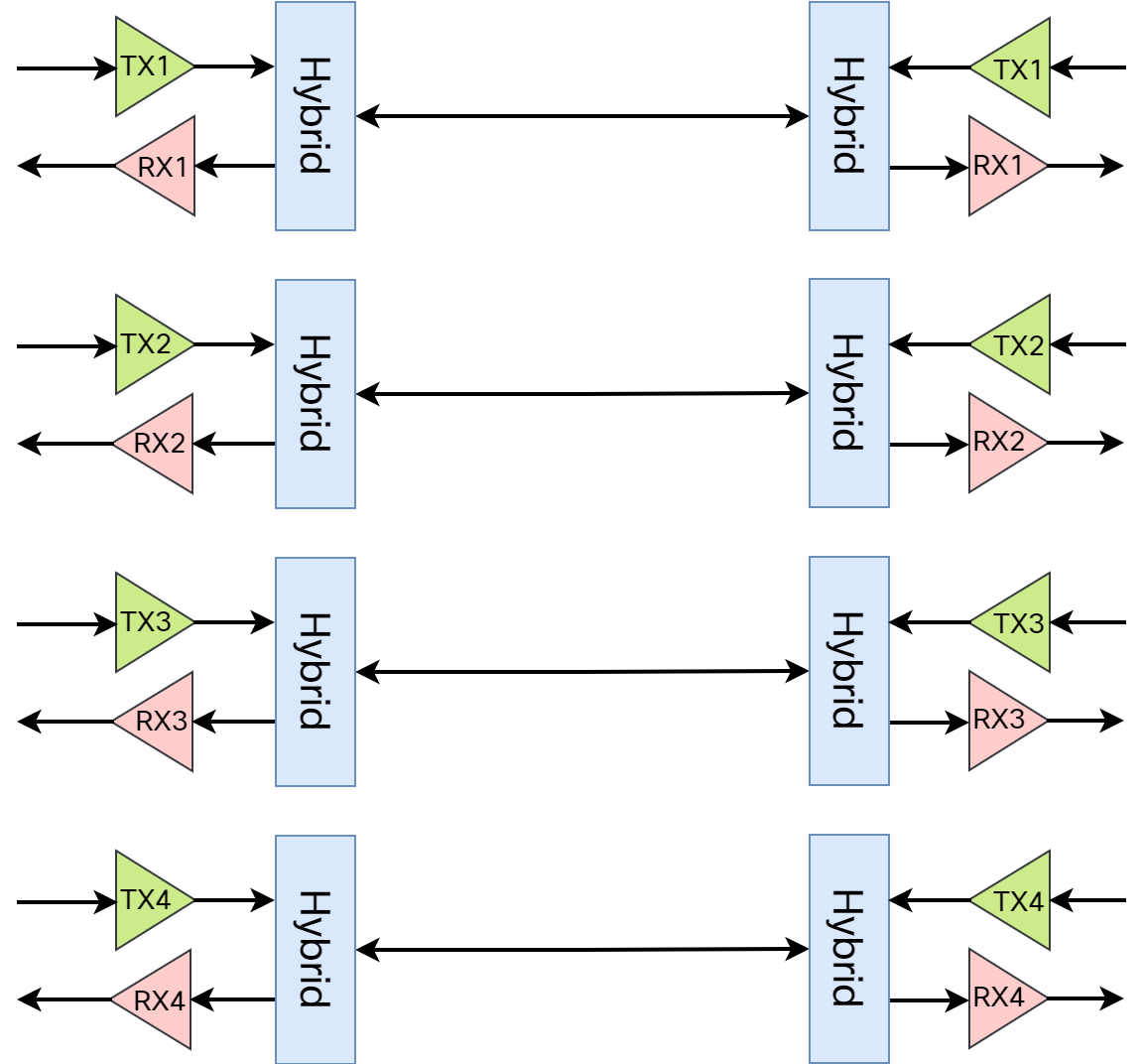
The meaning of hybrid in this context is that transmit and receive is performed on the same pair. Every pair is capable of 250 Mbit/s data rate, for a total of 1000 Mbit/s. As PAM-5 encoding is used (more on this later), the baud rate is 125 MHz. This means that the PHY receives 8-bit words to send every Continue reading
Tech Bytes: Simplifying Network Deployment & Operations With Nile (Sponsored)
Today Austin Hawthorne from Nile joins us to dig into the company’s Network as a Service (NaaS) approach and how it differentiates from traditional networking solutions. Nile aims to streamline network deployment and operations by providing a complete network service: It performs the site survey, provides the switches and access points, brings the gear on... Read more »NB472: HPE Adds GenAI to Aruba Central; Intel Eager to Slurp Billions in Subsidies
Take a Network Break! This week we try to peel back the layers on HPE’s announcement about new GenAI capabilties in Aruba Networking Central, parse Broadcom’s touting of its AI credentials, and feel conflicted about Intel sucking up billions in taxpayer dollars. South Korean chipmaker SK Hynix dangles a $4 billion investment promise to the... Read more »Network Service Providers Hit with AI Traffic Surge
The growing use of AI by enterprises and consumers is impacting data center and provider networks. As such, both need to be upgraded to support growing AI traffic.Nornir Network Automation

Nornir is a Python library designed for Network Automation tasks. It enables Network Engineers to use Python to manage and automate their network devices. Unlike tools like Ansible which rely on domain-specific languages, Nornir leverages the full power of Python, giving you more flexibility and control over your automation scripts.
Nornir feels like what you'd get if Ansible and Python had a baby. If you're used to Ansible, you know that you first set up your inventory, write tasks, and execute them on all or selected devices concurrently. Nornir operates similarly, but the big difference is you use Python code instead of any Domain Specific Language.
My Life Without Nornir
Before I discovered Nornir, my approach to Python automation involved manually setting up a list of devices, specifying each one's vendor, and credentials. This setup could be a simple Python list or a dictionary. Then, I'd loop through each device with a for loop, using libraries like Netmiko or Napalm to execute tasks. These tasks ranged from getting data from the devices to sending configurations. Here is a very simple snippet of managing the devices and using them with Netmiko. This method can get complicated very easily once you start Continue reading
Repost: EBGP-Mostly Service Provider Network
Daryll Swer left a long comment describing how he designed a Service Provider network running in numerous private autonomous systems. While I might not agree with everything he wrote, it’s an interesting idea and conceptually pretty similar to what we did 25 years ago (IBGP without IGP, running across physical interfaces, with every router being a route-reflector client of every other router), or how some very large networks were using BGP confederations.
Just remember (as someone from Cisco TAC told me in those days) that “you might be the only one in the world doing it and might hit bugs no one has seen before.”
5G Crowd Analytics in Public Venues: What IT Leaders Need to Know
Verizon is demoing crowd analytics technology that uses 5G along with AI and mobile edge computing to give stadium operators insights into the flow of fans throughout a venue.HN727: Kubernetes Networking Essentials
Where there are containers, there is networking. Today we dig into the networking that underlies Kubernetes, the open source orchestration platform for container-based applications. Our guest Karim El Jamali takes us through the essential concepts: Nodes, pods, clusters, CNIs, virtual ethernet pairs, ingress controller, eBPF, and service meshes. As container-based applications grow in popularity, it’s... Read more »Copilot Not Autopilot

I’ve noticed a trend recently with a lot of AI-related features being added to software. They’re being branded as “copilot” solutions. Yes, Microsoft Copilot was the first to use the name and the rest are just trying to jump in on the brand recognition, much like using “GPT” last year. The word “copilot” is so generic that it’s unlikely to be to be trademarked without adding more, like the company name or some other unique term. That made me wonder if the goal of using that term was simply to cash in on brand recognition or if there was more to it.
No Hands
Did you know that an airplane can land entirely unassisted? It’s true. It’s a feature commonly called Auto Land and it does exactly what it says. It uses the airports Instrument Landing System (ILS) to land automatically. Pilots rarely use it because of a variety of factors, including the need for minute last-minute adjustments during a very stressful part of the flight as well as the equipment requirements, such as a fairly modern ILS system. That doesn’t even mention that use of Auto Land snarls airport traffic because of the need to hold other planes outside Continue reading
Public Videos: Service Insertion in EVPN Fabrics

In 2020, Lukas Krattiger ran a short webinar describing how to insert L4-L7 services into EVPN fabrics. The videos are now public, and you can view them without an ipSpace.net account.
Use AGW for packet radio applications
When creating packet radio applications, there are several options on how to get the packets “out there”, and get them back. That is, how to interface with the modem.
Sure, you can write your own modem, and have the interface to the outside world be plain audio and PTT (push to talk, i.e. trigger transmit). But now you’re writing a modem, not an application. You should probably split the two, and have an interface between them.
KISS
You can use KISS, but it’s very limited. You can only send individual packets, so it’s only really good for sending unconnected (think UDP) packets like APRS. It’s not good for querying metadata, such as port information and outstanding transmit queue.
Think of KISS like a lower layer that applications shouldn’t think about. Like ethernet. Sure, as a good engineer you should know about KISS, but it’s not what your application should be interfacing with.
Linux kernel implementation
On Linux you can use AF_AX25 sockets, and program exactly like you
do for regular internet/IP programs. SOCK_DGRAM for UI frames
(UDP-like), and SOCK_STREAM for connected mode (TCP-like).
But the Linux kernel implementation is way too buggy. SOCK_STREAM
works kinda OK, but does Continue reading